FCurves are 1 dimensional function curves constructed from 2D bezier functions.
They are often used to control a property over time.
x values don't have any units, but they often represent a duration in seconds.
The language to express FCurves is similar to SVG's path language.
| Relative command | Absolute command | Description |
|---|---|---|
m y |
M y |
move the pen only in the y-direction |
h x |
hold a value to draw a horizontal line | |
H x |
shift curve in time by x. Can only be used as first command. | |
l x,y |
L x,y |
line to (x, y) |
q x0,y0,x,y |
Q x0,y0,x,y |
quadratic bezier to (x,y) and control-point (x0, y0) |
c x0,y0,x1,y1,x,y |
C x0,y0,x1,y1,x,y |
cubic bezier to (x,y) and control-points (x0, y0), (x1, y1) |
t x,y |
T x,y |
quadratic smooth to (x, y) |
s x1,y1,x,y |
S x1,y1,x,y |
cubic smooth to (x,y) and control point (x1, y1) |
This is an example of a flat horizontal FCurve:
// set the initial value to 0.5, hold that value for 1 seconds
val sizeCurve = fcurve("M0.5 h1")
Two horizontal segments at different heights:
// hold value 0.4 for half second, then hold value 0.6 for half second
val sizeCurve = fcurve("M0.4 h0.5 M0.6 h0.5")
Note that x values are relative, except for H where x is absolute.
For y values, lower case commands are relative and upper case commands are absolute.
We can interpolate from height 0.2 to 0.8 in 2 seconds like this:
// set initial value to 0.2, then interpolate linearly to value 0.8 over 2 seconds
val sizeCurve = fcurve("M0.2 L2,0.8")
Easily visualize the curves by calling the .contours() method. It will convert
the curve into a list of ShapeContour instances which are easy to draw using
drawer.contours():
val sizeCurve = fcurve("M0.2 L2,0.8")
drawer.contours(sizeCurve.contours())Note that the bounding box of this last curve will have a width of 2.0 pixels and a height under 1.0 pixel.
In other words, almost invisible at its original scale.
Since this is a common situation the .contours() method accepts a
Vector2 scale argument to control the rendering size:
val sizeCurve = fcurve("M0.2 L2,0.8")
drawer.contours(sizeCurve.contours(Vector2(drawer.width / sizeCurve.duration, drawer.height.toDouble())))The Q and C commands (and their lowercase counterparts) allow us to draw quadratic (one control point)
and cubic (two control points) curves.
// A quadratic curve that starts at zero, with a control point at 1,0 and ending at 1,1.
// That's a curve that stays near the 0.0 value and quickly raises to 1.0 at the end.
val easeOutCurve = fcurve("M0.0 Q1.0,0.0,1.0,1.0")

// A cubic s-shaped curve spending more time at both ends with a quick transition between them in the middle.
val easeInOutCurve = fcurve("M0.0 C1,0,0,1,1,1")
Note that new lines, white space and commas are optional. They can help with readability:
M0 h10
c 3,10 5,-10 8,0.5
L 5,5
The T and S commands (and their lowercase counterparts) allow us to create smooth curves, where
one control point is automatically calculated to maintain the curve direction. The smooth curve
commands require the presence of a previous segment, otherwise the program will not run.
// Hold the value 0.5 during 0.2 seconds
// then draw a smooth curve down to 0.5, up to 0.7 down to 0.3 and up to 0.7
val smoothCurveT = fcurve("M0.5 h0.2 T0.2,0.3 T0.2,0.7 T0.2,0.3 T0.2,0.7")

// Hold the value 0.5 during 0.2 seconds
// then draw a smooth with 4 repetitions where we move up slowly and down quickly
val smoothCurveS = fcurve("M0.5 h0.2 S0.2,0.0,0.2,0.5 S0.2,0.0,0.2,0.5 S0.2,0.0,0.2,0.5 S0.2,0.0,0.2,0.5")
Useful methods provided by FCurve:
smoothCurveS.reverse()returns a new reversed FCurve.smoothCurveS.changeSpeed(0.5)returns a new FCurve scaled horizontally.smoothCurveS.durationreturns the duration of the FCurve.
Drawing FCurves is useful for debugging, but their typical use is for animation. The FCurve sampler allows us to query values for the given time value like this:
fun main() {
    application {
        program {
            val xCurve = fcurve(
                """
                M320 H0.4
                S2,0, 2,320
                S2,0, 2,320
                S2,0, 2,320
                S2,0, 2,320
                T0.6,320
                """.trimIndent()
            ).sampler() // <--
            extend {
                drawer.circle(
                    xCurve(seconds % 9.0),
                    height * 0.5,
                    20.0
                )
            }
        }
    }
}
In this example we used % 9.0 to loop the time between 0.0 and 9.0, repeating the animation over and over.
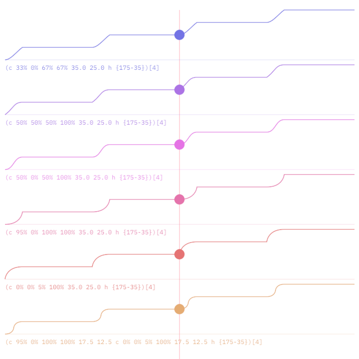
Extended Fcurves have an additional preprocessing step in which scalar expressions are evaluated.
EFCurves support comments using the # character.
M0 h10 c3,10,5,-10,8,0.5 # L5,5
M0 h10               # setup the initial y value and hold it for 10 units.
c3,10,5,-10,8,0.5    # relative cubic bezier curve
# and a final line-to
L5,5
Expressions within curly brackets are evaluated using orx-expression-evaluator.
Please refer to its documentation for details on the expression language used.
For example: M0 L{3 * 4},4 evaluates to M0 L12,4.
EFCurves add support for repetitions. Repetitions are expanded by replacing
occurrences of (<text-to-repeat>)[<number-of-repetitions>] with number-of-repetitions copies
of text-to-repeat.
For example:
M0 (h1 m1)[3]expands toM0 h1 m1 h1 m1 h1 m1M0 (h1 m1)[0]expands toM0
Repetitions can be nested.
For example (M0 (h1 m1)[3])[2] expands to M0 h1 m1 h1 m1 h1 m1 M0 h1 m1 h1 m1 h1 m1.
M0 (H{it + 1} m1)[3] expands to M0 H1 m1 H2 m1 H3 m1
M0 (H{index + 1} m{it}){1.2, 1.3, 1.4} expands to M0 H1 m1.2 H2 m1.3 H3 m1.4


